Building a Two-Wheeled Balancer with LQR Control

About the Project

Our aim is to design a two-wheeled balancer, and program a self-balancing robot that uses LQR control to maintain its upright position. The project integrates concepts from linear algebra, state space equations, Lagrangian mechanics, and control theory, along with 3D modeling, MATLAB simulations, and stepper motor control with ESP-IDF.

Lagrangian Mechanics

Instead of focusing on forces and Newton’s laws, Lagrangian mechanics uses the Lagrangian function, \(L\), which is the difference between the kinetic energy \(T\) and potential energy \(V\) of a system: \[ L = T - V \]

The Lagrangian approach is better because we don’t need to know the forces but just the constraints and we can straightforwardly use any type of coordinates we want as long as they describe the system. Equations of motion are obtained by using the Euler-Lagrange equation: \[ \frac{d}{dt}\left(\frac{\partial L}{\partial \dot{q}_i}\right)-\frac{\partial L}{\partial q_i} = 0 \] Where \(q_i\) are the generalized coordinates.

Control System

Control means to regulate or direct. Thus, a control system is the interconnection of various physical elements connected in a way to regulate or direct itself or the other system.

State Space System

A system to be controlled is described in state-space form as: \[ \dot{x} = Ax + Bu \] Where \(x\) represents the state variables, \(\dot{x}\) their rate of change, \(u\) is the control input from actuators, matrix \(A\) describes the system dynamics (how states interact), and \(B\) describes how inputs affect the states.

The output equation is: \[ y = Cx + Du \] Where \(y\) is the output vector, \(C\) maps state variables to outputs, and \(D\) represents any direct feedthrough from inputs to outputs. This representation allows us to model and analyze the system's behavior.

LQR Control

Now we know how to represent a system to be controlled. LQR stands for Linear Quadratic Regulator, designed for linear systems to minimize a quadratic cost function. The cost function \(J\) is: \[ J = \int_{0}^{\infty} (x^T Q x + u^T R u) dt \] Here, \(Q\) is a positive semi-definite matrix penalizing state deviations (error), and \(R\) is a positive definite matrix penalizing control effort.

The optimal control law that minimizes \(J\) is a state feedback law: \[ u = -Kx \] Where \(K\) is the optimal gain matrix, calculated as \( K = R^{-1}B^TP \). The matrix \(P\) is the unique positive definite solution to the Algebraic Riccati Equation (ARE): \[ A^TP + PA - PBR^{-1}B^TP + Q = 0 \] Uff, enough maths let’s get to implementation.

Implementation in MATLAB

Let’s try to model an inverse pendulum on a cart using LQR control.

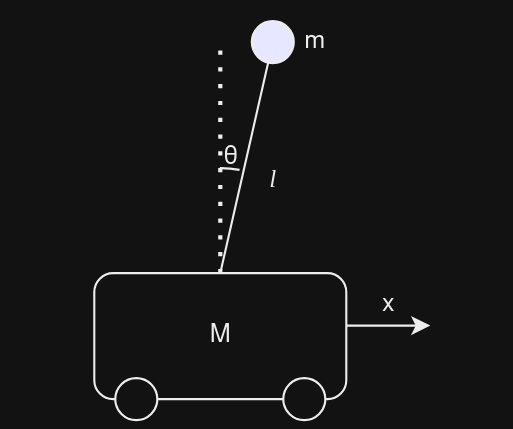
Free Body Diagram of Inverted Pendulum on Cart — Inverted Pendulum on Cart FBD

Using Lagrangian mechanics, the kinetic energy \(T\) and potential energy \(V\) are derived. The Lagrangian \(L = T - V\) for this system (assuming cart mass \(M\), pendulum mass \(m\), pendulum length \(l\)) is approximately: \[ L = \frac{1}{2}(M+m)\dot{x}^2 + \frac{1}{2}m( l^2\dot{\theta}^2 + 2l\dot{x}\dot{\theta}\cos(\theta) ) - mgl\cos(\theta) \] Applying the Euler-Lagrange equations yields the non-linear equations of motion. To linearize them, we consider the equilibrium point where the pendulum is upright (\(\theta = 0\), \(\dot{\theta} = 0\)) and the cart is at rest (\(\dot{x} = 0\)). Using small angle approximations (\(\cos\theta \approx 1\), \(\sin\theta \approx \theta\)) and neglecting higher-order terms, we get the linearized equations: \[ (M+m)\ddot{x} + ml\ddot{\theta} = u \\ ml\ddot{x} + ml^2\ddot{\theta} - mgl\theta = 0 \] Which can be rearranged to solve for \(\ddot{x}\) and \(\ddot{\theta}\) to form the state-space model.

My state variables here are \([x, \theta, \dot{x}, \dot{\theta}]^T\). Let's set an initial position \(x(0)=2\) (with other states zero) and a desired final position \(x_{final}=-2\).

The LQR controller will calculate the force \(u\) on the cart required to move it to \(x=-2\) while keeping the pendulum balanced (\(\theta \approx 0\)).

Putting all this in MATLAB and simulating gives us a controlled output like this:

Simulation of Inverted Pendulum Control — MATLAB Simulation: Inverted Pendulum Stabilization

The simulation shows the cart moving to the target position while the pendulum remains balanced.

Relation of \(Q\) and \(R\)

As we saw earlier, LQR tries to minimize the cost function involving the weighting matrices \(Q\) and \(R\). These matrices allow us to tune the controller's behavior. Let's consider a simple pendulum example (not inverted) trying to reach \(\theta = -\pi/2\) from rest (\(\theta = 0\)). The states are \([\theta, \dot{\theta}]^T\).

Base Case: Equal Penalty (Q = diag([100, 100]), R = 0.001)

Here, errors in position (\(\theta\)) and velocity (\(\dot{\theta}\)) are penalized equally. Control effort (\(u\)) is penalized very little.

Base Case Simulation — Base Case: Equal Penalty

More Penalty on Position Error (Q = diag([100, 1]), R = 0.001)

The controller focuses more on reducing the angle error quickly, potentially at the cost of higher velocity or overshoot.

Higher Q(1,1) Simulation — Emphasis on Position Accuracy

More Penalty on Control Effort (Q = diag([100, 100]), R = 1)

The controller tries to be "lazy," using minimal torque (\(u\)) to reach the target, resulting in slower movement.

Higher R Simulation — Emphasis on Control Effort Minimization

Key Takeaway: Increasing elements in Q makes the system prioritize reducing state deviations (faster, more aggressive control).

Key Takeaway: Increasing R makes the system prioritize minimizing control effort (slower, more conservative control, potentially allowing larger state deviations).

In practical robotics, balancing performance (speed, accuracy) with actuator effort (energy consumption, hardware limits) is crucial. Tuning Q and R allows engineers to find this balance for specific application requirements.

3D Model and Specifications

We created a 3D model of our balancer using Onshape. For control, we plan to use NEMA17 stepper motors for precision, driven by A4988 drivers (Note: original text mentioned A2988, A4988 is more common). An ESP32-WROOM microcontroller will run the control algorithm developed using the ESP-IDF framework.

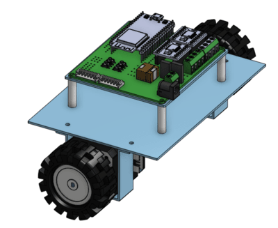
3D CAD Model of the Balancer Robot — Balancer CAD Model (Onshape)

This CAD model helps visualize the physical system and can eventually be used for more detailed simulations (e.g., Simscape Multibody in MATLAB).

Updates

Completed understanding basics of Control Systems and LQR.
Successfully simulated control of Pendulum, Spring-Mass system, and Inverted Pendulum.
Finished initial CAD Model for the balancer.

Challenges

Achieving precise stepper motor control with high-frequency updates in ESP-IDF.
Correctly deriving and validating the state-space matrices (A, B) for the physical robot.
Integrating sensor fusion (e.g., Kalman filter for IMU data) effectively.
Bridging the gap between simulation results and real-world hardware performance.

Future Plans

Refine the mathematical model and simulate the balancer CAD model in MATLAB/Simulink.
Implement and test Kalman filtering for IMU sensor fusion on the ESP32.
Develop a robust stepper motor control library within ESP-IDF.
Deploy the LQR control algorithm on the ESP32 and begin real-world testing.