I’m working on a project of perception for which I will try to implement ORB-SLAM3, to build the knowledge for it, I have listed out few papers. This is the first paper leading me to it, I will try to explain this paper in detail. This was quite a catchy read, the paper did not feel boring or dragged out. Before reading this paper I was expecting it to be quite complex and something alien but it was an interesting read.
I got reminded of the old AR videos while reading this, there was quite a variety and I remember Ben10 being one of it, GeoGebra etc. As this paper was published in 2007, back then AR stuff relied on markers. The problem this paper aims to solve is the removal of those markers to build a 3D environment. However, they aim this for small workspaces, by splitting the tracking and mapping into 2 separate tasks to build a 3D map.
Section 2 - Overview of the method
Tracking and Mapping are separated, and run in two parallel threads
Mapping is based on keyframes, which are processed using batch techniques
In short, removing redundant frames and processing large batch of data at once (we will break this down in further sections)
The map is densely initialized from a stereo pair (5-Point Algorithm).
New points are initialized with an epipolar search.
Imagine you identify a new pixel in your current camera view that isn’t in the map yet. You want to find this same pixel in a previous keyframe to triangulate it and add it to the 3D map. Instead of searching the entire old image (which is slow), camera geometry tells you that the matching point must lie along a specific line in the old image. This line is called the epipolar line. Searching only along this line is much, much faster.
Large numbers (thousands) of points are mapped.
Map
Central Hub
Single instance
System controller
MapPoint
3D World Points
2K-6K points
8×8 patches
Keyframe
Camera Snapshots
40-120 frames
4-level pyramid
Map Class
The Map is the central container for the entire 3D world representation. Its sole function is to hold and manage the collections of all recognized MapPoints and selected Keyframes.
classMap { List<MapPoint> points; List<Keyframe> keyframes; function add_point(new_point); function add_keyframe(new_keyframe);
}
MapPoint Class
A MapPoint represents a single, triangulated 3D point in the world. It stores its 3D position and surface orientation (normal vector).
Key Function: Each MapPoint maintains a direct reference to the specific Keyframe it was originally detected in, including the image pyramid level and pixel patch coordinates.
classMapPoint {
int id; Vector4 position_in_world; Vector3 normal_vector; Keyframe source_keyframe; int pyramid_level; Vector2 patch_coordinates_in_source;
}
Keyframe Class
A Keyframe is a snapshot of the camera at a specific, informative moment. It stores the camera's exact pose (its transformation from the world coordinate system) and the multi-resolution image data from that moment.
classKeyframe { int id; Matrix4x4 world_to_camera_transform; List<Image> image_pyramid;
}
This stored image pyramid serves as the source material from which new MapPoints are generated.
System Core
3D Features
Visual Data
Section 3 - Structure of the MAP
The first mathematical representation we come across is while defining the point feature, which is this: \[p_{j\mathcal{W}} = \begin{pmatrix} x_{j\mathcal{W}} \\ y_{j\mathcal{W}} \\z_{j\mathcal{W}} \\ 1\end{pmatrix}\] This basically tells the coordinate of \(j\)th point in the map \(p_j\) in World(\(\mathcal{W}\)) frame. Also each point is associated with a patch normal\(n_j\) and a reference to the patch source pixels. This \(n_j\) indicates the orientation of the real-world surface where the point was found.
The map stores \(N\) Keyframes. Each keyframe\(K_i\) contains a image pyramid, actual picture stored in multiple resolutions and its pose \(E_{kw}\) transformation between this coordinate frame and the world.
Section 4 - Understanding Tracking
The paper uses a “coarse-to-fine” strategy broken into 2 stages: Stage 1: Rough estimate Stage 2: refinement
Image Acquisition -
Constructs a 4 level image pyramid
Uses something called FAST-10 (Features from Accelerated Segment Test), without non-maximal suppression.
Now the 4 level image pyramid will come handy later on. Let us see FAST-10 in short.
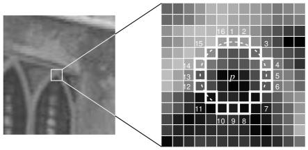
The FAST algorithm checks a circle of 16 pixels around a center pixel.
FAST aims at finding corners in an image to track them. It does it by choosing a pixel, looks at a circle of 16 pixels around it. If it finds a continuous arc of 10 or more pixels that are all significantly brighter or all significantly darker than the center pixel, it calls the center pixel a “corner.” Now FAST will often detect multiple corners right next to each other in a small cluster.
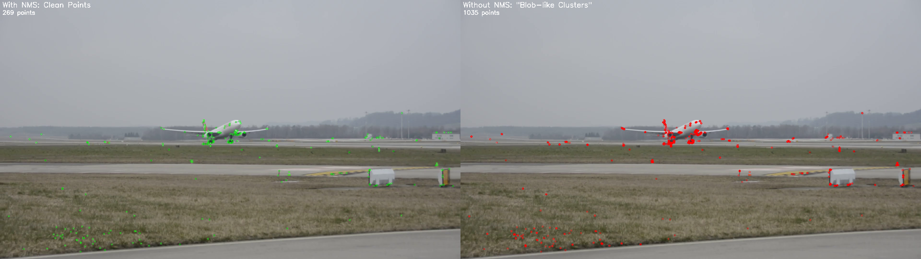
- WITHOUT Non-Maximal Suppression - You keep all the corners that pass the FAST test. This is what the paper means by “blob-like clusters of corner regions.” The result is dense and messy.
- WITH Non-Maximal Suppression - This is a cleanup step. basically choosing a dominant corner inn this case. Here is an example -
Keypoints found WITHOUT NMS: 1035 vs WITH NMS: 269
Camera Pose and Projection - The first equation we come across is: \[p_{j\mathcal{C}}=E_\mathcal{CW}*p_\mathcal{jW}\] What it says is that the coordinates of point \(j\) in the Camera frame (\(p_{j\mathcal{C}}\)) are equal to the camera pose matrix (\(E_\mathcal{CW}\)) multiplied by the coordinates of point \(j\) in the World frame.
When I read this the \(E_\mathcal{CW}\) just didn’t feel right, shouldn’t the camera’s pose be its position in the world?
But the \(E_\mathcal{CW}\) answers a question that from the camera’s perspective, where does this 3D point appear on my 2D screen? To do that, we need to know where every point in the world is relative to the camera.
Equation 2: Camera Projection Model \[\begin{pmatrix}u_i \\ v_i\end{pmatrix}=\text{CamProj}(E_\mathcal{CW}*p_\mathcal{iW})\]\[\text{CamProj}\begin{pmatrix}x \\ y \\ z\\ 1\end{pmatrix}=\begin{pmatrix}u_0 \\ v_0\end{pmatrix} + \begin{bmatrix}f_u & 0\\ 0& f_v\end{bmatrix}\frac{r'}{r}\begin{pmatrix}\frac{x}{z} \\ \frac{y}{z}\end{pmatrix}\]\[r=\sqrt{\frac{x^2+y^2}{z^2}}\]\[r'=\frac{1}{\omega}\arctan(2r\tan\frac{\omega}{2})\] This function takes a 3D point that is already in the camera’s coordinate system and calculates the final 2D pixel coordinates where it will appear in the image.
\(f_u\), \(f_v\) being the focal lengths in the x and y directions. \(u_0, v_0\) is the pixel coordinate of a point near to center.
Real lenses are not perfect, \(r\) calculates how far the 3D point is from camera’s central axis of view, \(r'\) is to accommodate the distortion. Updating the camera pose is done by \(E'_{\mathcal{CW}}= M* E_{\mathcal{CW}}=\exp(\mu)E_{\mathcal{CW}}\) .
Patch Search - A patch from original keyframe will look different in current frame. It might be rotated, scaled, or skewed due to perspective changes. Simply looking for the original pixels will fail. The system calculates a 2x2 matrix A called the affine warp matrix. \[A=\begin{bmatrix}\frac{\partial{u_c}}{\partial u_s}& \frac{\partial{u_c}}{\partial v_s} \\ \frac{\partial{v_c}}{\partial u_s}&\frac{\partial{v_c}}{\partial v_s}\end{bmatrix}\] Basically, it says \(\frac{\partial{u_c}}{\partial u_s}\), how much does the horizontal pixel coordinate in the current frame change if I move one pixel horizontally in the source frame… and so on for all 4.
We take a tiny square on the source image plane, use the known 3D geometry to figure out what that square corresponds to on the real-world surface, and then project that real-world surface patch into the current camera view to see how it’s distorted.
Choosing the Right Pyramid Level - It is done by using \(\det{(A)}\) , determinant of the warp matrix A represents the area change. If det(A) = 4, it means one source pixel now covers an area of 4 pixels in the current full-resolution image. We choose the pyramid level \(l\) where the patch’s scale is closest to 1. The formula is \[\frac{\det{(A)}}{4^l}\] and it should be close to 1.
Pose update
Now that the system has a set \(S\) of successful matches, it can update camera’s pose. \[e_j=\begin{pmatrix}\hat{u_j} \\ \hat{v_j}\end{pmatrix}-\text{CamProj}(\exp(\mu)E_{\mathcal{CW}}*p_j)\]\(\begin{pmatrix}\hat{u_j} \\ \hat{v_j}\end{pmatrix}\) - This is the observed position. It’s where the patch search actually found the point in the 2D image. \(\text{CamProj}(...)\) - This is the predicted position. It’s where the point should be, according to the current camera pose guess. \(e_j\) - The reprojection error vector. It’s the 2D pixel difference between “where I saw it” and “where my current model predicts I should have seen it.”
Now our task is to minimize this error.
\[\mu'=\arg\!\min_{\mu}\sum_{j \in S}\text{Obj}\left(\frac{|e_j|}{\sigma_j},\sigma_T\right)\] We find the \(\mu\) such that the cost is minimized. Instead of just minimizing the raw pixel error, the robust function heavily down-weights the influence of outlier measurements. This prevents a few bad matches from corrupting the entire pose estimate.
Two-stage coarse-to-fine tracking
Use only 50 points at the coarsest pyramid levels. This is fast and finds a rough pose even with large camera movements.
The second stage uses upto 1000 points. With the good pose estimate from the coarse stage, you only need to search a tight region in the finer pyramid levels.
Tracking quality and failure recovery Just a failsafe that when quality is poor, tracking continues, but the system is forbidden from adding new keyframes to the map. If the tracking is lost, the system does not continue.
This was the working of tracking thread. Now we can move on to mapping.
Section 5 - Understanding Mapping
This runs in a continuous, asynchronous loop along with Tracking thread.
Initialisation - System grabs first keyframe, finds ~1000 corners and these are the points to track. However, it relies on user to move sideways a bit and on second keyframe the points tracked their exact 3D rotation and translation using 5 point Algorithm.
But the initial map has 2 problems, system knows the camera moved, but it doesn’t know if it moved 10cm or 10 meters and the world’s coordinate system is aligned with the first camera view, which is not very useful.
To solve this we take 2 simple assumptions, we assume the user moved the camera 10cm and find the dominant plane in the point cloud using RANSAC, then rotate the entire world model so that this plane lies perfectly at \(z\)=0.
Keyframe Insertion - A new keyframe is added only if all these conditions are met -
The Tracking thread must be confident in its current pose.
At least 20 frames have passed since the last keyframe was added.
The camera’s current position must be a minimum distance away from the nearest existing keyframe in the map.
Once a new keyframe is integrated, the Map thread’s primary job is to find new 3D points to add to the map. The Tracking thread has already found a bunch of FAST corners in the new keyframe. The Map refines this list to find the most “salient” (stable, high-quality) corners that are not already observations of existing map points.
A new 3D point needs two views to be triangulated. The Map looks through all the past keyframes and finds the one that provides the best “stereo baseline” (a good side-view with enough parallax) for the new keyframe. For each candidate 2D point in the new keyframe, the system performs an epipolar search to find its match in the chosen partner keyframe. If a confident match is found, the new 3D point is triangulated and added to the global map.
Bundle adjustment - This is the key step in refining our pose, it aims to cure drift by optimizing the entire map and camera history at once, it tries to consistently map global coordinates. The text establishes the ultimate goal, captured in this equation \[\{\{\mu_2...\mu_N\},\{p'_{1}...p'_{M}\}\}=\mathop{\mathrm{argmin}}_{\{\{\mu\}, \{p\}\}}\sum_{i=1}^N\sum_{j\in S_i}\text{Obj}\left(\frac{|e_ji|}{\sigma_ji},\sigma_T\right)\] It states that the system should adjust all camera poses (\(E_1\) to \(E_N\)) and all 3D map points (\(p_1\) to \(p_M\)) simultaneously to minimize the total reprojection error across every single measurement ever made. This is Global Bundle Adjustment.
Problem is this is incredibly demanding, this is slow if if the camera is actively exploring a new area and adding new keyframes rapidly.
To solve this problem, a Local Bundle Adjustment method is used. Instead of optimizing the entire world, this version focuses only on a small, relevant “neighbourhood” of the map. \[\{\{\mu_{x\in X}\},\{p'_{z\in Z}\}\}=\mathop{\mathrm{argmin}}_{\{\{\mu\}, \{p\}\}}\sum_{i\in X \cup Y}^N\sum_{j\in Z\cap S_i}\text{Obj}\left(i,j\right)\]
\(X\) - The change now focuses on the most recent keyframe and its four closest neighbours. These are the poses that will be actively tweaked.
\(Z\) - The system adjusts all 3D map points that are visible in any of those five core keyframes.
\(Y\) - To prevent this local patch from drifting away from the rest of the stable map, the optimization also includes measurements from other keyframes that see the points in Z. However, the poses of these anchor keyframes are held fixed. They act as a rigid reference, tethering the local adjustment to the global map.
Data Association Refinement - What does the Map do when there are no new keyframes to process and the map has already been bundle-adjusted? It uses its free time to improve the quality of the map’s data. Two main tasks are performed -
When a new 3D point is created, it’s only linked to two keyframes, this point might have been visible in other, older keyframes too, but was never measured. The Map goes back to these other keyframes and actively searches for the new point. If it finds it, it adds this new measurement link to the map.
The outliers in cost functions are ignored, they are given a second chance and once again filtered to fit.
Pretty confusing, right? A lot to keep track of, but the main gist is that the Tracking thread figures out where the camera is, while the Mapping thread builds and refines the world.
Let us see overall summary of both threads.
Section 6 - Summary
Tracker thread
Acquire Image & Initial Guess
Grab a frame
Convert it to 4 level image pyramid
Estimate prior pose \(E_{\mathcal{CW}}\) for this frame. This is your starting guess.
Coarse Tracking Stage
Take a small subset of map points (~50) from the Map. Use \(p_{j\mathcal{C}}=E_\mathcal{CW}*p_\mathcal{jW}\) with your prior pose to transform them into the camera’s 3D space.
Use the CamProj() function to project these 3D camera-space points onto the image plane, finding their predicted 2D pixel coordinates (\(u\), \(v\)).
For each projected point, search for its corresponding visual patch in the coarsest (smallest) image pyramid level.
To do this, you first need to calculate the affine warp matrix \(A\)
Use the ~50 successful coarse matches to perform an initial pose update. This involves minimizing the reprojection error \(e_j=\begin{pmatrix}\hat{u_j} \\ \hat{v_j}\end{pmatrix}-\text{CamProj}(\exp(\mu)E_{\mathcal{CW}}*p_j)\).
Fine Tracking Stage
Take a much larger number of map points (~1000).
Use the new, improved E_cw from the coarse stage to transform and project them onto the image plane. Pretty much like the above step.
For each of these points, search for its patch in the finer (higher-resolution) pyramid levels. Because your pose estimate is now much better, you only need to search in a very small pixel radius.
Use all the successful matches from both the coarse and fine stages to run a final, robust pose optimization, resulting \(E'_{\mathcal{CW}}\) is the final, accurate pose for this frame.
Mapping thread
Initialisation - All the capturing keyframe and triangulation.
Main loop -
Is there a new keyframe in queue?
YES -
Add new features, find new corners, epipolar search and triangulation
Local bundle adjustment.
NO -
Run Global Bundle adjustment
That was the full breakdown of how the tracking and mapping threads work together to estimate camera pose and build a consistent 3D map. In the coming days, I will try to implement the entire paper or a part of it. If you’ve read this far, hopefully it made the paper a little more digestible. Thank you!